
PyTorchにおけるFocal Lossの実装を行ない、簡単な追試を行ない性能がどのようになるか見ていきます。
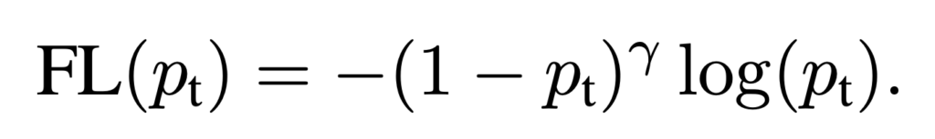
Focal Lossについて
Facebook AI Research (FAIR)によって2017年に物体検出を対象に提案された損失関数です。
「物体検出におけるR-CNNなどの2段階手法に比べて、1段階手法は高速な一方で性能が劣る課題があった。この性能が劣る理由は、クラス間の不均衡であることを発見し、これを解決するためにFocal lossを提案した。この損失関数を組み込んだネットワークを提案し、既存の2段階検出器の性能を超えつつ、一段階検出器と同等の速度を達成した。」
論文の概要は上記のような内容で、ここでFocal Lossが使われています。Focal Lossは、分類が容易なサンプルの重みを下げることで、分類が難しいサンプルにより焦点をあてる。これにより、サンプル数が少ないクラスや分類が難しいサンプルに対して学習がしやすくなる特徴があります。
Focal Lossは物体検出を対象に提案されたロス関数ですが、シンプルな形であり様々な分野やタスクに応用可能です。
マルチラベルを対象としたFocal Loss
マルチラベル分類タスクを対象としたFocal Lossを実装していきます。
import torch
from torch import nn
class Focal_MultiLabel_Loss(nn.Module):
def __init__(self, gamma):
super(Focal_MultiLabel_Loss, self).__init__()
self.gamma = gamma
self.bceloss = nn.BCELoss(reduction='none')
def forward(self, outputs, targets):
bce = self.bceloss(outputs, targets)
bce_exp = torch.exp(-bce)
focal_loss = (1-bce_exp)**self.gamma * bce
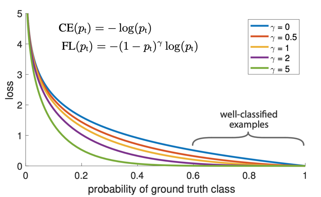
return focal_loss.mean()実装が正しいか確認するために、Binary Cross Entropy(BCE)と比較します。Focal Lossのγは2に指定します。
import matplotlib.pyplot as plt

# binary cross entropy
loss = nn.BCELoss(reduction='none')
target = torch.Tensor([1])
for input in torch.arange(0.001, 1, 0.001):
  output = loss(input, target[0])
  plt.scatter(input, output, color = "blue")

# focal loss γ=2
loss = Focal_MultiLabel_Loss(gamma=2)
for input in torch.arange(0.001, 1, 0.001):
  output = loss(input, target[0])
  plt.scatter(input, output, color = "red")

plt.xlabel('probability of ground truth class')
plt.ylabel('loss');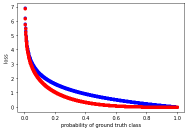
青線がBCEの結果で、赤線がFocal lossの結果になります。論文の図と同様になっていることが確認できました。
Focal Lossの効果の確認
Focal Lossの効果の確認するために、Kaggleクレジットカード詐欺データセットをダウンロードを利用します。
import pandas as pd

raw_df = pd.read_csv('<https://storage.googleapis.com/download.tensorflow.org/data/creditcard.csv>')
display(raw_df.head())
データの不均衡を確認してみると、全体の14%とPositiveが非常に少ないことが分かります。
import numpy as np
neg, pos = np.bincount(raw_df['Class'])
total = neg + pos
print('Examples:\\n    Total: {}\\n    Positive: {} ({:.2f}% of total)\\n'.format(
    total, pos, 100 * pos / total))

# Examples:
#     Total: 284807
#     Positive: 492 (0.17% of total)
簡単な前処理及び訓練データと検証データに分割し、DataLoaderにセットします。
from sklearn.model_selection import train_test_split
from torch.utils.data import DataLoader
cleaned_df = raw_df.copy()

cleaned_df.pop('Time')

eps = 0.001
cleaned_df['LogAmount'] = np.log(cleaned_df.pop('Amount') + eps)

train_df, test_df = train_test_split(cleaned_df, test_size=0.2, random_state=0)

train_labels = np.array(train_df.pop('Class'))
test_labels = np.array(test_df.pop('Class'))

train_features = np.array(train_df)
test_features = np.array(test_df)

batch_size = 128

train_dataset = torch.utils.data.TensorDataset(torch.tensor(train_features).to(torch.float32), torch.tensor(train_labels.astype(np.float32)).unsqueeze(1))
val_dataset = torch.utils.data.TensorDataset(torch.tensor(test_features).to(torch.float32), torch.tensor(test_labels.astype(np.float32)).unsqueeze(1))
train_dataloader = DataLoader(val_dataset, batch_size=batch_size, shuffle=True)
val_dataloader = DataLoader(val_dataset, shuffle=False)
シンプルなニューラルネットワークを定義します。
import torch.nn as nn
import torch.nn.functional as F

class SimpleNet(nn.Module):
    def __init__(self):
        super(SimpleNet, self).__init__()
        self.fc1 = nn.Linear(29, 16)
        self.fc2 = nn.Linear(16, 8)
        self.fc3 = nn.Linear(8, 1)

    def forward(self, x):
        x = F.relu(self.fc1(x))
        x = F.relu(self.fc2(x))
        x = torch.sigmoid(self.fc3(x))
        return x
まずは、損失関数をBinary Cross Entropyにして、学習させ性能を見ていきます。
import torch.optim as optim

device = "cuda" if torch.cuda.is_available() else "cpu"
print(f"Using {device} device")

model = SimpleNet().to(device)

criterion = nn.BCELoss() # Binary Cross Entropy
optimizer = optim.Adam(model.parameters(), lr=1e-3)

def train(dataloader, model, loss_fn, optimizer):
    size = len(dataloader.dataset)
    model.train()
    for batch, (X, y) in enumerate(dataloader):
        X, y = X.to(device), y.to(device)

        # Compute prediction error
        pred = model(X)
        # print(X)
        # print(pred)
        # print(y)
        loss = loss_fn(pred, y)

        # Backpropagation
        optimizer.zero_grad()
        loss.backward()
        optimizer.step()

        if batch % 100 == 0:
            loss, current = loss.item(), batch * len(X)
            print(f"loss: {loss:>7f}  [{current:>5d}/{size:>5d}]")

epochs = 2
for t in range(epochs):
    print(f"Epoch {t+1}\\\\n-------------------------------")
    train(train_dataloader, model, criterion, optimizer)
print("Done!")
学習したモデルで検証データを推論し、混同行列を見てみます。
from sklearn.metrics import confusion_matrix
import seaborn as sns

pred = []
Y = []
model.eval()
for x, y in val_dataloader:
    with torch.no_grad():
        output = model(x.to(device))
    pred += [1 if output > 0.5 else 0]
    Y += [int(l) for l in y]

# 混同行列表示用
def plot_confusion_matrix(true, predicted):
    cm = confusion_matrix(true, predicted)
    fig, ax = plt.subplots(figsize = (10,10))
    sns.heatmap(cm, square=True, cbar=False, annot=True, cmap='Blues')
    plt.xlabel("Predicted label")
    plt.ylabel("True label")

plot_confusion_matrix(Y, pred)
全てのデータをモデルが0と予測していることが分かります。
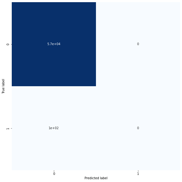
次に、損失関数にFocal Lossを設定したモデルで検証データを推論し、混同行列を見てみます。
model = SimpleNet().to(device)

criterion = Focal_MultiLabel_Loss(gamma=4) # Binary Cross Entropy
optimizer = optim.Adam(model.parameters(), lr=1e-3)

for t in range(epochs):
    print(f"Epoch {t+1}\\\\n-------------------------------")
    train(train_dataloader, model, criterion, optimizer)
print("Done!")

pred = []
Y = []
model.eval()
for x, y in val_dataloader:
    with torch.no_grad():
        output = model(x.to(device))
    pred += [1 if output > 0.5 else 0]
    Y += [int(l) for l in y]

plot_confusion_matrix(Y, pred)

少数派のラベルに対しても推論が上手くいっていることが確認できました。
コメント